Pair approximation
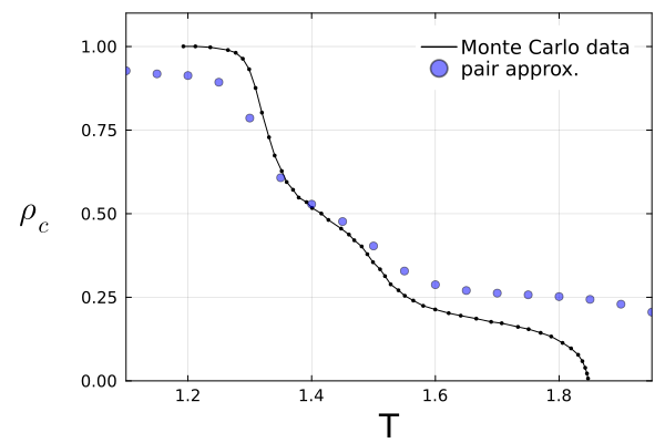
In structured populations, finding analytical results is extremely difficult. Normally, models of evolutionary dynamics in lattices resort to Monte Carlo simulations. Pair approximation is one approach to try to replicate them, but via differential equations, without the need to run simulations (hauert2005).
Lets focus on pairs of interacting players $p_{A,B}$, and all pairs connecting them The figure below shows an illustration of that, where x,y,z denotes the three connections of A and u,v,w the connections of B.
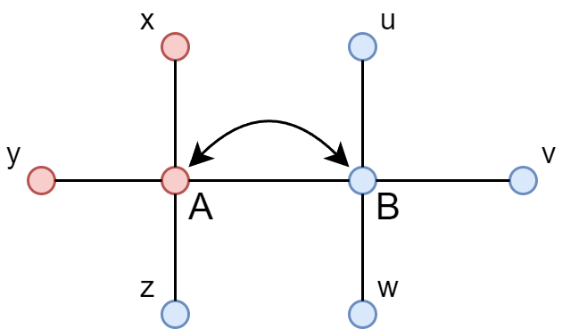
The transition probabilities are given by one strategy of a pair flipping $p_{A,B\rightarrow B,B}$, which is given by
\[\begin{align} p_{A,B\rightarrow B,B} = \sum_{x,y,z}\sum_{u,v,w} f(P_B - P_A) \times \frac{p_{x,A}\, p_{y,A}\,p_{z,A}\,p_{A,B}\,p_{u,B}\,p_{v,B}\,p_{w,B}}{p_A^3\,p_B^3} \end{align}\]where $f(P_B - P_A)$ is the probability of strategy adoption (normally the Fermi equation). In total we have six sums and all go from 0 to 1 to consider all possible neighborhoods of the pair (A,B). For example, $p_{x,A}$ can be $p_{0,A}$ ($p_{1,A}$) which is the probability of A having a defector (cooperator) as neighbor in the x direction.
In total, we would need four variables: $p_{c,c}$, $p_{d,d}$, $p_{c,d}$ and $p_{d,c}$. But since $p_{c,d} = p_{d,c}$ and $p_{c,c} + p_{d,d} + p_{c,d} + p_{d,c} = 1$, we need two differential equations, that are given by
\[\begin{align} \dot{p}_{c,c} = \sum_{x,y,z} \, [n_c(x,y,z)+1]\,p_{d,x}\,p_{d,y}\,p_{d,z} \sum_{u,v,w} p_{c,u}\,p_{c,v}\,p_{c,w}\,f(P_c(u,v,w)-P_d(x,y,z)) \\ - \sum_{x,y,z} \, n_c(x,y,z)\, p_{c,x}\,p_{c,y}\,p_{c,z}\sum_{u,v,w} p_{d,u}\,p_{d,v}\,p_{d,w}\, f(P_d(u,v,w)-P_c(x,y,z)) \end{align}\] \[\begin{align} \dot{p}_{c,d} = \sum_{x,y,z} \, [1 - n_c(x,y,z)]\,p_{d,x}\,p_{d,y}\,p_{d,z} \sum_{u,v,w} p_{c,u}\,p_{c,v}\,p_{c,w}\,f(P_c(u,v,w)-P_d(x,y,z)) \\ - \sum_{x,y,z} \, [2 - n_c(x,y,z)]\, p_{c,x}\,p_{c,y}\,p_{c,z} \sum_{u,v,w} p_{d,u}\,p_{d,v}\,p_{d,w}\, f(P_d(u,v,w)-P_c(x,y,z)) \end{align}\]The changes always come from a (d,c) interaction, since we are using imitation. In both equations, the first term is related to a defector changing to cooperation, and the second term a cooperator changing to defection.
Considering that the pair (A,B) changes from (d,c) to (c,c)
- we get $1+n_c$ new (c,c) and $1-n_c$ new (d,c) pairs
Considering that the pair (A,B) changes from (d,c) to (d,d)
- we lose $n_c$ pairs (c,c) and $2-n_c$ new (d,c) pairs
Code
1
2
3
4
5
6
7
8
9
# C. Hauert, S. György, Game theory and physics, Am. J. Phys. 73, 405 (2005)

#         x        u
#         |        |
#         |        |
# y ----- A ------ B ------ v
#         |        |
#         |        |
#         z        w
Parameters
1
2
3
4
5
6
7
8
9
10
11
12
13
using Plots, Printf,HomotopyContinuation, LinearAlgebra, DelimitedFiles, PlutoUI

begin
    const K = 0.1
    const k = 4
    const R = 1.0
    #const T = 1.1
    const P = 0.0 #not used
    const S = 0.0 #not used

    # HomotopyContinuation
    @var ρcc ρcd
end
Definitions
1
2
3
4
5
6
7
8
9
10
11
function W_fermi(ΔP, K)
    return 1.0 / (1.0 + exp(-ΔP / K))
end

function payoff_C(nc, R, S)
    return  (nc+1)*R + (k - nc)*S
end

function payoff_D(nc, T, P)
    return  (nc+1)*T + (k - nc)*P
end
Master eq.
1
2
3
4
5
6
7
8
9
10
11
12
13
14
15
16
17
18
19
20
21
22
23
24
25
26
27
28
29
30
31
32
33
34
35
36
37
38
39
40
41
42
43
44
45
46
function calculo_pho(ρ⃗, params)

    T, R, P, S, K = params

    eq_cc = 0.0
    eq_cd = 0.0

    #    ρ₁₁ ρ₁₂  -> ρdd  ρdc
    #    ρ₁₂ ρ₂₂  -> ρcd  ρcc

    p = [1.0-(ρ⃗[1]+2*ρ⃗[2])      ρ⃗[2];
                 ρ⃗[2]              ρ⃗[1]]

    for x in 0:1 # todas configuraçoes possiveis (D = 0 e C = 1)
        for y in 0:1
            for z in 0:1
                for u in 0:1
                    for v in 0:1
                        for w in 0:1

                            nc_xyz = x + y + z
                            nc_uvw = u + v + w

                            Pc_xyz = payoff_C(nc_xyz, R, S)
                            Pc_uvw = payoff_C(nc_uvw, R, S)
                            Pd_xyz = payoff_D(nc_xyz, T, P)
                            Pd_uvw = payoff_D(nc_uvw, T, P)

                            Wcd = W_fermi(Pc_uvw - Pd_xyz, K)
                            Wdc = W_fermi(Pd_uvw - Pc_xyz, K)

                            A₁ = p[1,1+x]*p[1,1+y]*p[1,1+z]*p[2,1+u]*p[2,1+v]*p[2,1+w] #ρdi  ρcj
                            A₂ = p[2,1+x]*p[2,1+y]*p[2,1+z]*p[1,1+u]*p[1,1+v]*p[1,1+w] #ρci  ρdj

                            eq_cc += (nc_xyz+1)*A₁*Wcd - nc_xyz*A₂*Wdc
                            eq_cd += (1-nc_xyz)*A₁*Wcd - (2-nc_xyz)*A₂*Wdc

                            #@printf "%d %d %s\n" nc_xyz nc_uvw A₁
                        end
                    end
                end
            end
        end
    end
    return eq_cc, eq_cd
end
Soluton
1
2
3
4
5
6
7
8
9
10
11
12
13
14
15
16
17
18
19
20
21
22
23
24
25
26
27
28
29
30
31
32
33
34
35
36
37
38
39
final_solutions = []
#T = 1.5
for T in 1.0:0.05:3.0

    params = [T; R; P; S; K]

    ρ⃗ = [ρcc; ρcd]

    eq_cc, eq_cd = calculo_pho(ρ⃗, params)

    # use HomotopyContinuation solve to solve polynomial system of equations
    F = System([eq_cc,eq_cd])
    result = solve(F; start_system = :polyhedral)

    # filtering solutions
    num_solutions = size(real_solutions(result))[1]
    real_sol = real_solutions(result) # in function of ρcc
    selected_solutions = Float64[] # in function of ρc now

    # testar estabilidade com jacobiano simbólico
    for i in 1:num_solutions
        ρ₁₁, ρ₁₂ = real_sol[i]     # ρcc, ρcd
        ρc = ρ₁₁ + ρ₁₂             # ρcc + ρcd
        ρd = 1.0 - ρc
        #@printf "%f %f\n" ρc ρd

        if ((0.0 ≤ ρ₁₁ ≤ 1.0) && (0.0 ≤ ρ₁₂ <= 1.0) && (ρc ≤ 1.0)
            && (0.0 ≤ ρd ≤ 1.0))
            push!(selected_solutions, ρc)

            re_eigs = real(eigvals(jacobian(F,[ρ₁₁,ρ₁₂])))

            if re_eigs[1]<-1E-10 && re_eigs[2]<-1E-10
                push!(final_solutions, (T, ρc))
            end
            @printf "---> %f %8.6f %8.6f %8.12e %8.12e\n" T ρc ρd re_eigs[1] re_eigs[2]
        end
    end
end